Plot ESR spectra and peak finding

Function to plot an ESR spectrum and finding peaks using an automated routine.

plot_Spectrum(data, stacked = FALSE, normalise = FALSE, crop = TRUE,
  y_scale_factor = 2, vertical_lines, vertical_lines_manual,
  col_bg = "grey90", manual_shift, manual_shift_global, gvalue = FALSE,
  difference = FALSE, integrate = FALSE, smooth.spline = FALSE,
  smooth.spline.df, smooth.spline.diff.df, overlay = TRUE,
  auto.shift = FALSE, shift.method = "ccf", find.peaks = FALSE,
  peak.range, peak.threshold = 10, peak.information = FALSE,
  info = NULL, plot = TRUE, add = FALSE, ...)

Arguments

data	`data.frame` (required): data frame with two columns for x=magnetic.field or g.value, y=ESR.intensity.
stacked	`logical` (with default): If `TRUE` this function produces a stacked plot where each spectrum is plotted on top of each other. Use `y_scale_factor` to adjust the y-axis scaling. Defaults to `FALSE`.
normalise	`logical` (with default): If `TRUE` each spectrum is normalised by its individual maximum intensity value. This is useful to compare the spectrums structure by eliminating relative intensity variations. Requires `stacked = TRUE`. Defaults to `FALSE`.
crop	`logical` (with default): If `TRUE` all spectra are cropped to the specified `xlim` range before applying any further signal processing (e.g. normalisation). Useful when plotting spectra with different scan widths. Defaults to `TRUE`.
y_scale_factor	`numeric` (with default): A positive single numeric value that determines the scaling of the y-axis when `stacked = TRUE`. Lower values will bring the spectra closer to each other, potentially making them overlap each other. Increasing the value will increase the distance and flatten the spectra. Defaults to `2`.
vertical_lines	`numeric` (optional): Add vertical dashed lines at specified x-axis values. See `abline()`.
vertical_lines_manual	`list` (optional): A `list` of vectors of `numeric` values to draw custom vertical lines in the plot. Each vector should be of the same length as the number of spectra provided. Each value indicates where a vertical line is drawn in the spectrum, starting from the bottom to the top. Example: `data` is a list with three spectra. To connect the three spectra with a vertical line use e.g. `vertical_lines_manual = list(c(3455, 3460, 3456))`. Useful, if the spectra are not perfectly aligned and you want to connect a particular are of interest with lines.
col_bg	`character` (with default): If more than one spectrum is provided the background is `grey90` by default.
manual_shift	`numeric` (optional): If all of the `auto.shift` methods fail to properly align all of the provided spectra use `manual_shift` to align them manually. This should be a vector of negative or positive `numeric` values the same length as the number of provided spectra. Example: `data` is a list with three spectra. To shift the spectra use e.g. `manual_shift = c(-2, 0, 0.2)`, which aligns the first spectrum by `-2` to the left and the third by `0.2` to the right.
manual_shift_global	`numeric` (optional): The same as `manual_shift`, but shifting all spectra by one single value. Useful to shift spectra according to a calibration measurement. The correction is applied after individual shifts of `manual_shift`, so it is possible to individually AND globally shift the spectra for proper alignment.
gvalue	`logical` (with default): If `TRUE` and all spectra are of class `ESR.Spectrum` with information on microwave frequency the magnetic field values are converted to g-values.
difference	`logical` (with default): plot first derivative of the spectrum
integrate	`logical` (with default): plot integrand of the spectrum
smooth.spline	`logical` (with default): fit a cubic smoothing spline to supplied spectrum.
smooth.spline.df	`integer`: desired number of degrees of freedom
smooth.spline.diff.df	`integer`: desired number of degrees of freedom for splines of the first derivative
overlay	`logical` (with default): overlay actual data and smoothing spline curve in one plot.
auto.shift	`logical` (with default): automatically shift multiple spectra by their maximum peak. This uses smoothing splines for better results.
shift.method	`character` (with default): when `integral` the peaks are shifted by the maximum intensity of the integral. Alternatively, `deriv` can be used to shift the spectra by the minimum of the first derivative. By default, `ccf` is used which computes the cross-correlation of two univariate series (see `ccf`).
find.peaks	`logical` (with default): find and plot peaks (`TRUE/FALSE`).
peak.range	`integer` (with default): range of magnetic field intensities or g-values in which peaks are picked from `c(from, to)`. If no values are provide the whole spectrum is analysed.
peak.threshold	`integer` (with default): threshold value specifying the resolution of the peak finding routine (see details).
peak.information	`logical` (with default): plot peak intensity values for peaks found by the automated routine (`TRUE/FALSE`). Applies only when `find.peaks = TRUE`.
info	`character`: add information on experimental details as subtitle
plot	`logical` (with default): show plot (`TRUE/FALSE`).
add	`logical` (with default): whether derivatives and/or integrands are added to the spectrum or are shown separately (`TRUE/FALSE`).
...	Further plot arguments to pass.

Value

Returns terminal output and a plot. In addition, a list is returned containing the following elements:

data

list containing the (modified) input data

splines

list containing the spline objects

auto.peaks

data frame containing the peak information (magnetic field and ESR intensity) found by the peak find routine.

Details

Status

In progress

Note

In progress

Examples



##load example data
data(ExampleData.ESRspectra, envir = environment())

##plot dpph and use the automatic peak finding routine
plot_Spectrum(ExampleData.ESRspectra$dpph, find.peaks = TRUE,
                 peak.range = c(3340,3355),
                 peak.threshold = 10, peak.information = TRUE,
                 verbose = TRUE)
#>   magnetic.field ESR.intensity
#> 1       3345.623       6277086
#> 3       3347.969        -20205
#> 2       3350.237      -6257030

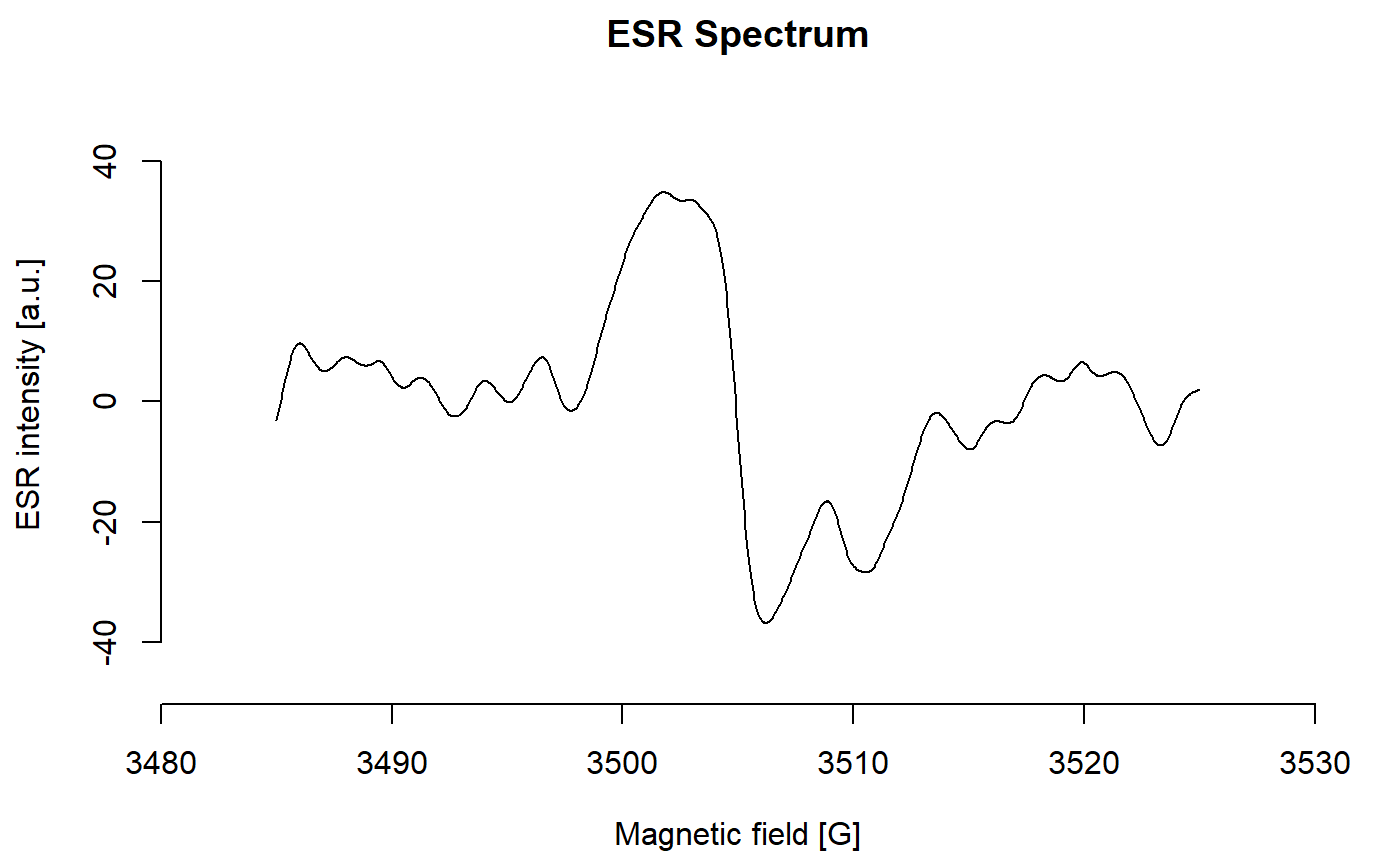
##plot the mollusc (sample Ba01) natural ESR spectrum with a smoothing spline
plot_Spectrum(ExampleData.ESRspectra$Ba01_00,
                 smooth.spline = TRUE,
                 smooth.spline.df = 40,
                 overlay = TRUE)

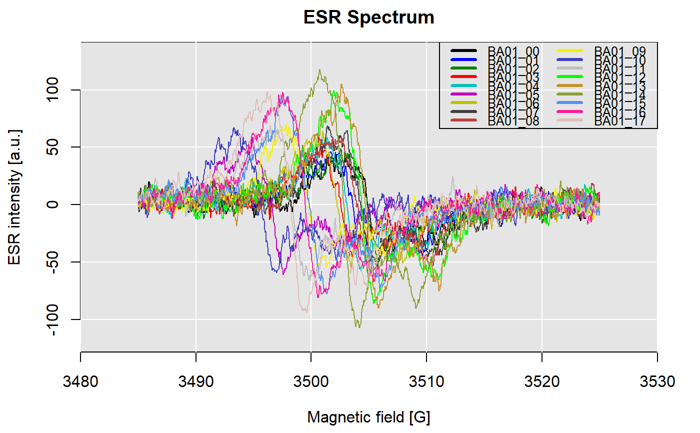
##plot all ESR spectra of sample Ba01
plot_Spectrum(ExampleData.ESRspectra$Ba01)

##plot all ESR spectra of sample Ba01 and align curves by the max peak
plot_Spectrum(ExampleData.ESRspectra$Ba01,
                 auto.shift = TRUE)

##plot all ESR spectra of sample Ba01, use smoothing splines and
##align curves by the max peak
plot_Spectrum(ExampleData.ESRspectra$Ba01,
                 smooth.spline = TRUE,
                 smooth.spline.df = 40,
                 auto.shift = TRUE,
                 overlay = FALSE)

Arguments

Value

Details

Note

See also

Examples

Contents

Author